Also posted in Microsoft Blog for PostgreSQL
Same Query, Same Index, Different Performance
I recently worked with a customer planning a migration from on-premises PostgreSQL to Azure Database for PostgreSQL. During performance testing, they noticed something troubling: a query that completed in tens of milliseconds would now take 1-2 seconds in the Azure environment being evaluated.
The query was using an index scan, and running it again was fast. But once the relevant data was evicted from cache, the long execution time came back. Naturally, the conversation turned toward storage performance. There was a clear difference in IOPS consumption, with the to-be-production server having 10-20% more IOPS consumption than a server they stood up for comparison purposes. A cold-cache query execution that performed a single Index Scan pulled over 100 pages from heap, whereas the other server only pulled 60 pages. The natural inclination was to think that somehow bloating and/or fragmentation was the cause, so they tried VACUUM FULL but did not see any improvement. That’s when they turned to us.
Is the Index Really the Problem?
The primary concern that the customer had – an Index Scan was not performing as well as expected – surfaced two hypotheses: something was wrong with the index, (i.e., bloat, leaf density, fragmentation), or something was wrong with the storage. Digging in with pg_stattuple and pg_statindex, we didn’t see anything glaringly wrong with leaf density or fragmentation. We also saw nothing from our telemetry that anything was wrong with the storage. With the usual suspects out of the picture, we needed to get back to the basic principles of indexing.
It is important to remember that when it comes to indexing a table, a regular index scan uses the index to locate matching tuples, then visits the table’s heap pages to retrieve them. The index is ordered; the heap doesn’t have to be.
Suppose a query returns 200 rows. If those rows live on five heap pages, Postgres can retrieve them with relatively little page access. If they are scattered across 100 pages, retrieving the same 200 rows requires a much larger working set. Both queries can say Index Scan in the execution plan, but that doesn’t mean they do equivalent work.
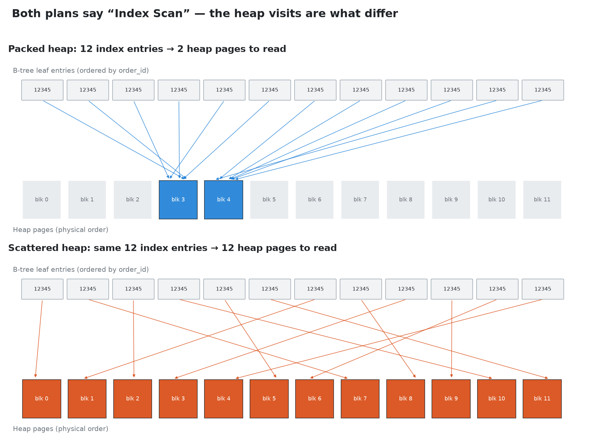
We compared EXPLAIN (ANALYZE, BUFFERS) output, looking beyond the scan type to buffer hits and reads. One caveat: a shared-buffer read means the page wasn’t in PostgreSQL’s shared buffers, not necessarily that it came from physical storage – the operating system may still have it cached. I/O timings, when track_io_timing is enabled, help distinguish cheap reads from expensive ones.
Small Hint: Look at Correlation
One useful clue was in pg_stats. Using generic table and column names here:
SELECT correlation FROM pg_stats WHERE schemaname = 'public' AND tablename = 'order_items' AND attname = 'order_id'; correlation describes how closely a column’s logical ordering follows the table’s physical ordering. Values near 1 or -1 indicate strong ordering; values near 0 indicate little relationship. Postgres uses this statistic when estimating index scan costs.
In this case, the slower environment had a correlation around 0.037, while the faster performance-test environment was around 0.571. That certainly suggested a layout difference!
But correlation is a sampled, column-wide statistic. It doesn’t tell us exactly how many heap pages contain the rows for one particular lookup. A table can have groups of related rows packed together without those groups appearing in globally sorted order. We needed to measure the thing the query actually cared about.
The Query That Made It Click
Postgres exposes a system column called ctid, which identifies a tuple’s physical location as (block_number, tuple_number). Extracting the block number lets us count the distinct heap pages containing our matching rows:
SELECT count(*) AS rows_found, count(DISTINCT split_part( trim(both '()' FROM ctid::text), ',', 1 )) AS distinct_heap_pages FROM public.order_items WHERE order_id = 12345; This example assumes an ordinary, non-partitioned table. For a partitioned table, count distinct (tableoid, block_number) pairs instead, since different partitions can have the same block numbers. Also, ctid is a diagnostic tool here, not a permanent row identifier – updates and table rewrites can change it.
For two representative lookup values, these were the actual counts, with the lookup values anonymized:
| Lookup | Rows returned | Slower environment: heap pages | Faster environment: heap pages |
|---|---|---|---|
| A | 157 | 119 | 33 |
| B | 200 | 101 | 5 |
There it was. For lookup B, the slower environment’s matching rows occupied about 20 times as many heap pages. These counts aren’t a complete accounting of query I/O – index pages and other accesses still matter – but they directly expose the heap footprint of the result.
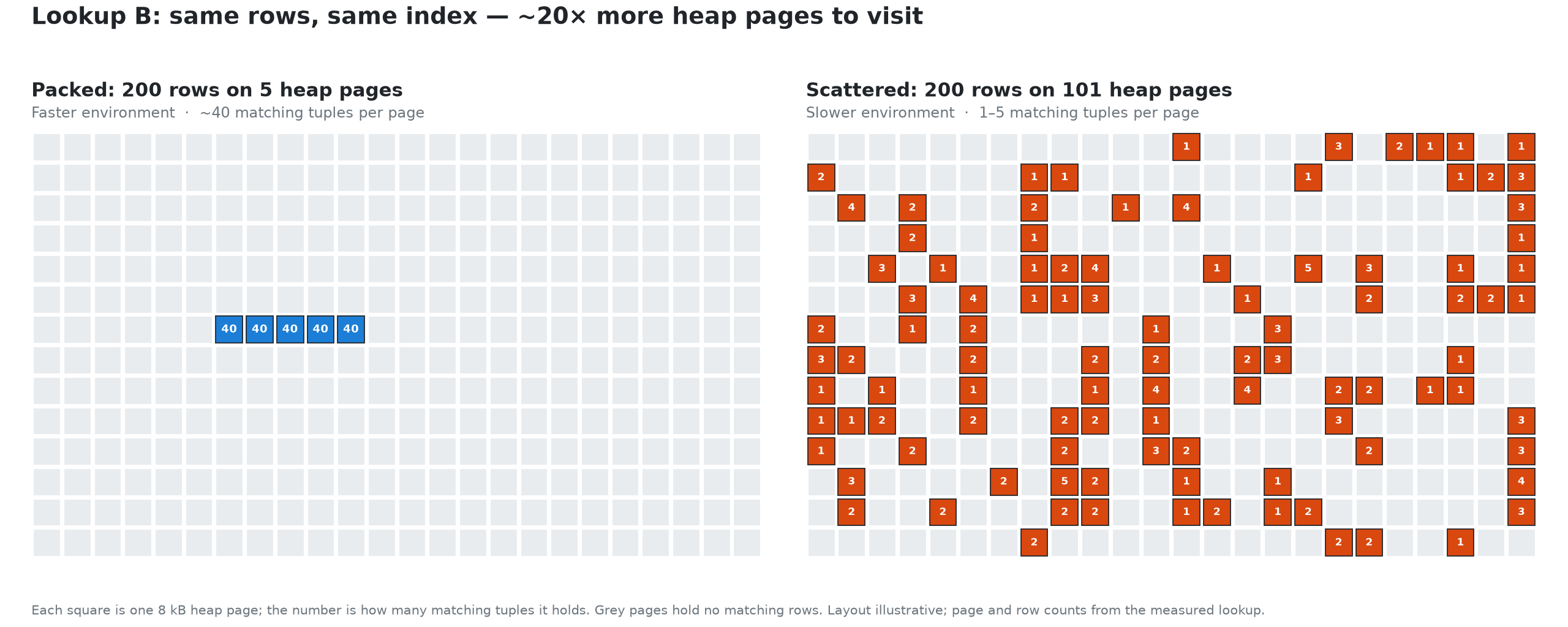
The index wasn’t failing to find the rows. The rows were simply spread across far more pages once it found them.
How Did the Rows Get So Scattered?
The customer had loaded data into the Azure environment in parallel. That helped load throughput, but the concurrent loading interleaved rows belonging to different lookup values. Related rows that had been packed together in the source environment no longer landed together in the destination heap.
Parallel loading doesn’t inherently guarantee a scattered table. The outcome depends on how work is divided and how inserts reach the heap. In this customer’s case, though, the loading method explained the observed layout difference.
Recreating the same index didn’t restore that locality. A B-tree orders its own entries; building or rebuilding it does not reorder the underlying table.
This also explained the cache behavior. Repeat executions benefited from cached pages, masking the cost of the larger footprint. Once those pages were evicted, the query had to fetch them again. More scattered data also meant more pages competing for cache space.
Fix the Layout, Then Measure Again
VACUUM FULL wouldn’t solve this layout problem, as it rewrites the table to reclaim space from dead tuples and compact the heap, but it doesn’t sort the surviving rows by the lookup key. It might reduce the page count if there is bloat, but related rows can still be interleaved with unrelated rows afterward. The issue here was less about fragmentation or bloat and more about which tuples were arranged together on disk.
The next step was to reorganize the heap around the lookup key. CLUSTER can rewrite a table in index order, but it takes an ACCESS EXCLUSIVE lock, so it needs careful scheduling. The customer used pg_repack with --order-by to reorganize the data and reported improved performance on a restored test instance.
That’s not a maintenance-free operation either: check extension support, free space, and locking requirements before choosing it. Afterward, refresh statistics with ANALYZE, repeat the distinct-page query, and compare execution plans and timings under comparable cache conditions. Running the diagnostic itself warms pages, so don’t treat the immediately following execution as a cold-cache test!
Neither clustering nor repacking permanently maintains the ordering. Future writes can erode locality, so the migration loading strategy and ongoing workload both deserve attention.
Final Thoughts
Before blaming storage latency, check how many pages each environment needs to read for the same query.
For this customer, correlation prompted us to examine the heap layout. Counting unique heap pages showed just how scattered the matching rows were. The lesson wasn’t “don’t load in parallel” or “Azure needs a bigger disk.” Migrating the same rows and indexes doesn’t necessarily migrate the same physical layout. An index scan is only half the story!


