Define metrics once and keep them correct with the dbt Semantic Layer on Amazon Redshift

Most analytics stacks model data into a curated gold layer and call the result a semantic layer. For a lot of workloads, that’s a perfectly good one. The business logic lives in version-controlled models, every consumer reads the same tables over SQL, and there’s no extra product to run. The honest position is that a well-modeled gold layer is a semantic layer for standardizing metrics, and reaching for a dedicated tool before you need one is over-engineering.

This post is about the point where that stops being true: when users need to compute a metric across arbitrary combinations of dimensions, chosen at query time, and some of those metrics are non-additive. We will first show, with real numbers, why pre-aggregated gold tables produce silently wrong results in that case. Then we will build a working solution on Amazon Redshift using the open-source dbt Semantic Layer (powered by MetricFlow), define average_order_value once, and prove it stays correct whether you slice it by day, by week, or by store.

A quick note on where this fits on AWS. Semantic and metric definitions on AWS have generally lived downstream of the warehouse rather than inside it. Amazon Quick Sight Topics define metrics for Quick Sight dashboards and Amazon Q. The newer AWS Context service builds a knowledge-graph layer over the AWS Glue Data Catalog to attach business meaning to data assets for agents and downstream tools (overview). Those are the places to watch as that story matures. This post stays deliberately narrow on a different, less-documented need: a governed metric layer you define once in Git, right next to your Amazon Redshift models, and query correctly from any tool. You build it with open-source dbt and MetricFlow.

The problem: Where a gold layer stops short

Limitation 1: The combinatorial wall

A gold table is pre-aggregated at one grain. To let users slice a metric by any combination of dimensions, you need a pre-built table per combination, and that count explodes as 2ⁿ:

Nobody builds 128 tables. You build the dozen someone asked for and field a ticket for every new slice. The escape hatch is to expose one wide fact table and let each business intelligence (BI) tool do its own GROUP BY. That restores flexibility, and it walks straight into the second, nastier problem.

Limitation 2: The metric is wrong, and nobody notices

Many everyday BI metrics are non-additive: you can’t roll them up by averaging the sub-totals. Average order value is the one nearly every dashboard has.

Suppose one store had these orders in a week:

Your gold table is pre-aggregated to a daily grain, because that’s what the daily sales dashboard needed:

Now someone asks a new question: “What was the average order value this week?” The BI tool only has the daily gold table, so it averages the two daily numbers:

($1,000 + $100) / 2 = $550 [WRONG] looks fine, is wrong

The real answer, from the actual orders, is:

total revenue / total orders = $1,400 / 5 = $280 [CORRECT] the truth

The naive rollup reports $550, nearly double the real $280. Nobody sees the error, because $550 is a plausible-looking number. The daily averages were each correct. Averaging them was the mistake. The weekly figure has to be recomputed as SUM(revenue) / COUNT(orders) at the week grain, and a pre-aggregated daily table doesn’t carry what’s needed to do that. Conversion rate, profit margin, cost per acquisition, and distinct counts all share this trap.

The requirement, then, isn’t “standardize the columns.” It’s: define the metric and its aggregation rules once, and compute them correctly on the fly for any dimensions a user picks. That’s exactly what the dbt Semantic Layer does, and the rest of this post builds it on Amazon Redshift.

Solution overview

We will put the metric definition in a dbt project, with Amazon Redshift as the warehouse. dbt builds the gold model. MetricFlow turns metric definitions in YAML into correct, grain-aware SQL at query time.

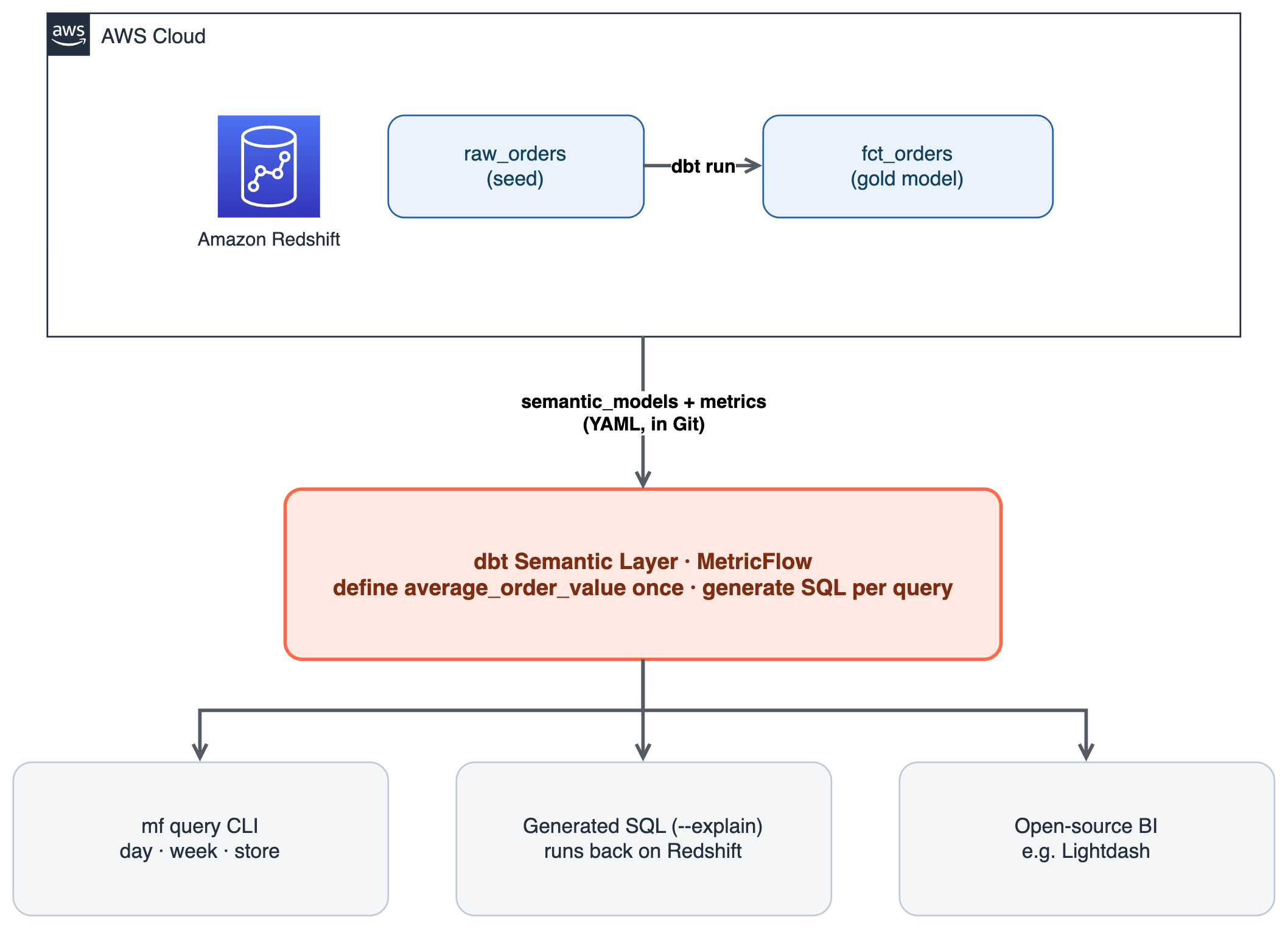
Figure 1: Architecture of the dbt Semantic Layer on Amazon Redshift

We keep the dataset deliberately tiny: only the five orders shown earlier. You can verify every number by hand and watch the week-grain result come back as $280, not $550.

The full dbt project and the AWS Cloud Development Kit (AWS CDK) app used in this walkthrough live in the companion repository, sample-dbt-semantic-layer-on-amazon-redshift: the dbt project under dbt/ and the Redshift Serverless CDK app under infra/. The repo also ships deploy, destroy, and end-to-end test scripts. See its README for a one-command runbook.

Prerequisites

• An AWS account with permission to create an Amazon Redshift Serverless workgroup (or an existing Amazon Redshift cluster) and query it.
• An Amazon Redshift database and schema you can write to, plus the connection endpoint, user, and password. (AWS Identity and Access Management (IAM), or IAM, authentication also works. This walkthrough uses a user and password for brevity.)
• Python 3.9–3.12 and pip.
• Basic familiarity with the command line and dbt.

Estimated cost: A Redshift Serverless workgroup with 8 RPUs (Redshift Processing Units) bills about $3/hour of active query time (metered per second, with a 60-second minimum per query), so a short walkthrough like this typically costs under a dollar. Follow the Clean up section to avoid ongoing charges.

Step 1: Provision Amazon Redshift and note the connection details

If you don’t already have an Amazon Redshift endpoint, create a Redshift Serverless workgroup from the console (Amazon Redshift → Redshift Serverless → Create workgroup). Note the workgroup’s endpoint, the database name (default dev), and the admin user and password you set.

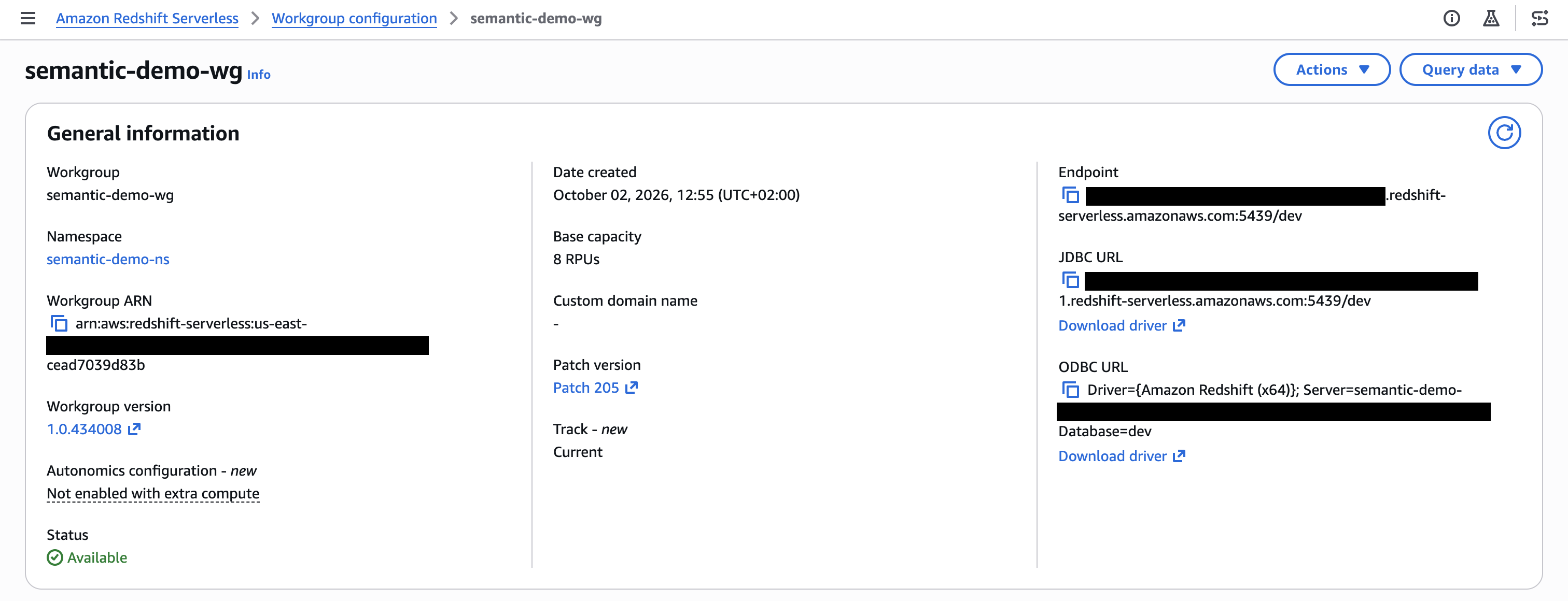
Figure 2: The Redshift Serverless workgroup detail page with its endpoint, port 5439, and database dev

If you prefer infrastructure-as-code, use the AWS CDK app in the companion repo’s infra/. Set your target account and AWS Region, then run the provided deploy script, which scopes inbound access to your current IP:

export CDK_DEFAULT_ACCOUNT=<your-account-id> CDK_DEFAULT_REGION=<your-region> ./scripts/deploy.sh

Read the generated admin password from AWS Secrets Manager (the script prints the secret name). An overly broad CIDR such as 0.0.0.0/0 is rejected unless you explicitly opt in. The preceding console steps remain valid.

Open Query Editor v2 and create a schema for this project:

CREATE SCHEMA IF NOT EXISTS semantic_demo;

Step 2: Set up the dbt project

Create and activate a virtual environment, then install the dbt adapter for Amazon Redshift and MetricFlow. Installing dbt-redshift brings a compatible dbt-core (1.9+ is required for the time-spine YAML used later), and dbt-metricflow adds the mf CLI:

python -m venv .venv source .venv/bin/activate pip install "dbt-redshift==1.9.5" "dbt-metricflow==0.11.0"

These versions are pinned so the walkthrough matches the output shown here. dbt-metricflow currently resolves dbt-core to the 1.10.x line. Newer dbt-core releases print a deprecation notice during dbt debug but behave the same for this project. If you prefer to stay current, install the latest dbt-redshift and dbt-metricflow. The metric definitions in Step 4 are unchanged.

Initialize a project:

dbt init aov_demo cd aov_demo

Want the exact runnable project used here instead of building from scratch? Clone the companion repo. Its dbt project and profile are both named semantic_demo. Copy dbt/profiles.example.yml to ~/.dbt/profiles.yml rather than running dbt init aov_demo. You can also reproduce the entire walkthrough end to end with ./scripts/e2e-test.sh.

Configure the connection in ~/.dbt/profiles.yml (replace the placeholders with your workgroup values):

aov_demo: target: dev outputs: dev: type: redshift host: <your-workgroup>.<account>.<region>.redshift-serverless.amazonaws.com user: admin password: "{{ env_var('REDSHIFT_PASSWORD') }}" port: 5439 dbname: dev schema: semantic_demo threads: 4 sslmode: require

Export the password and confirm the connection:

export REDSHIFT_PASSWORD='<your-password>' dbt debug

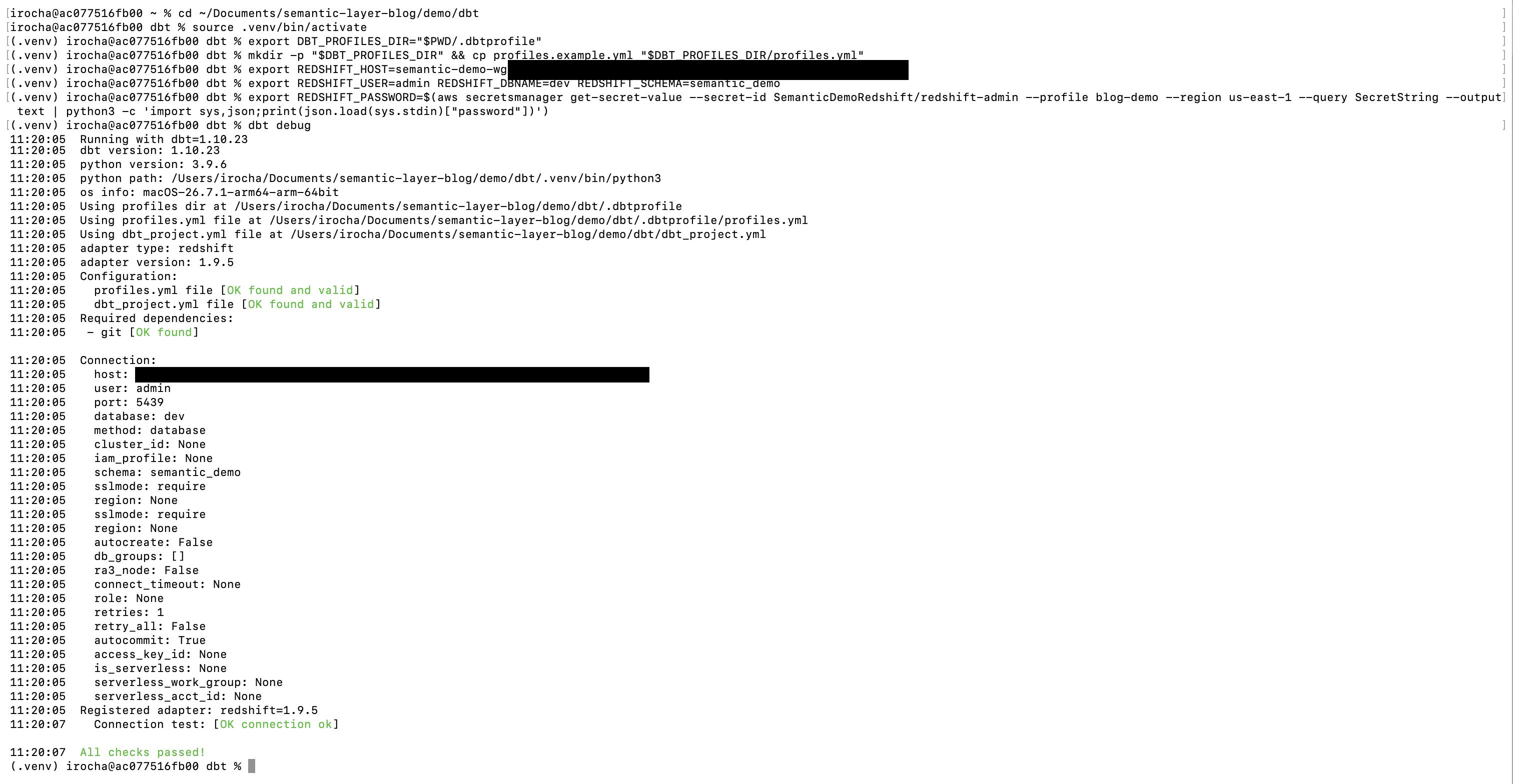
Figure 3: The dbt debug command confirms the Amazon Redshift connection, with all checks passing

Add dbt_utils (used for the time spine MetricFlow needs) in packages.yml:

packages: - package: dbt-labs/dbt_utils version: [">=1.0.0", "<2.0.0"]

dbt deps

Step 3: Seed the sample orders and build the gold model

Create seeds/raw_orders.csv with the exact five orders from the problem section (Jan 5, 2026 is a Monday and Jan 6 a Tuesday, in the same ISO week):

order_id,store,ordered_at,amount 1,downtown,2026-01-05,1000 2,downtown,2026-01-06,100 3,downtown,2026-01-06,100 4,downtown,2026-01-06,100 5,downtown,2026-01-06,100

Load it into Amazon Redshift:

dbt seed

Create the gold model models/marts/fct_orders.sql:

{{ config(materialized='table') }} select order_id, store, cast(ordered_at as date) as ordered_at, amount from {{ ref('raw_orders') }}

Create the time spine MetricFlow uses to reason about dates, models/marts/metricflow_time_spine.sql:

{{ config(materialized='table') }} with days as ( {{ dbt_utils.date_spine( datepart="day", start_date="cast('2026-01-01' as date)", end_date="cast('2026-02-01' as date)" ) }} ) select cast(date_day as date) as date_day from days

Register the time spine in models/marts/_models.yml:

models: - name: metricflow_time_spine time_spine: standard_granularity_column: date_day columns: - name: date_day granularity: day

Build everything:

dbt run

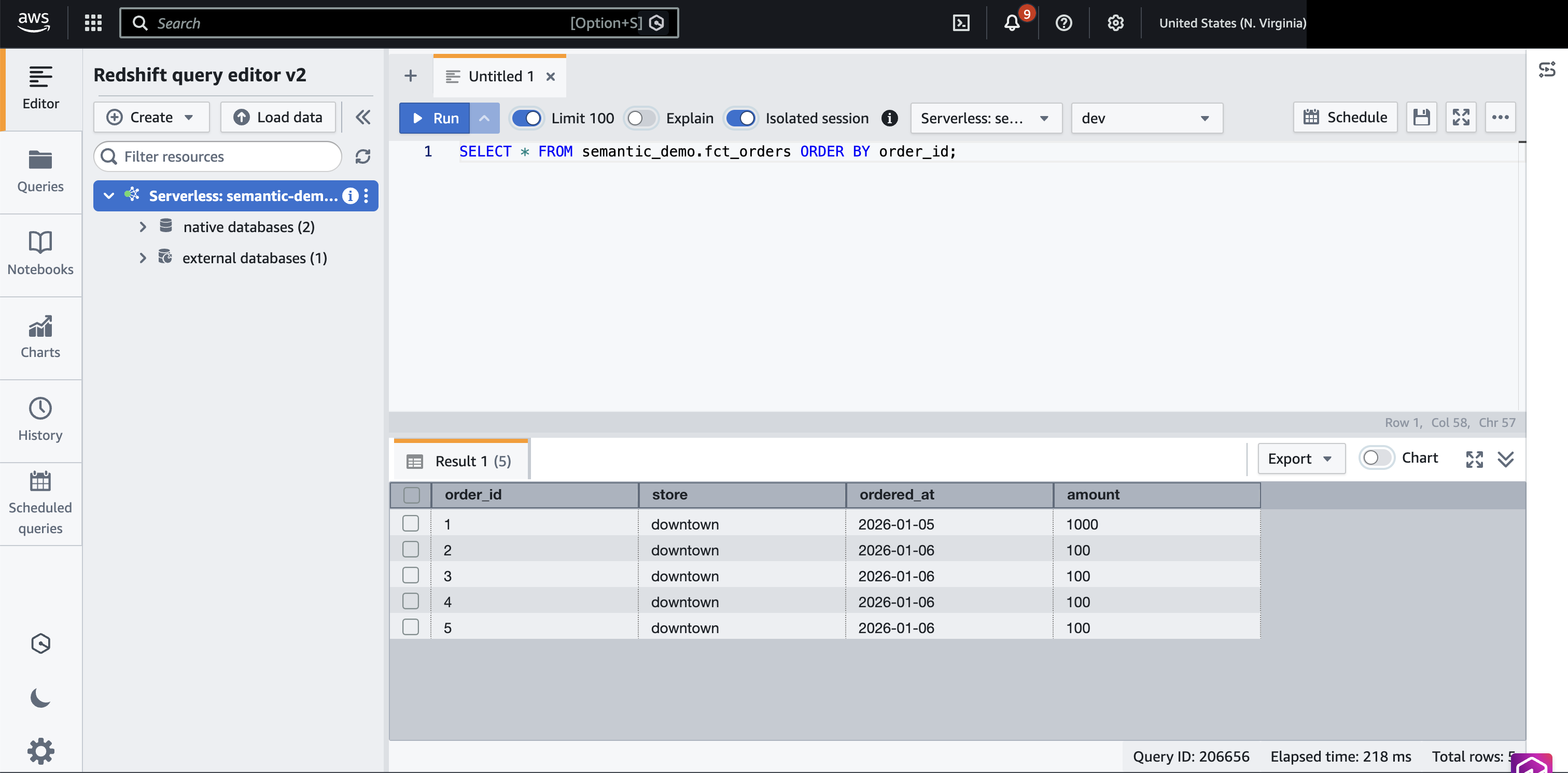
Figure 4: The five seeded orders in the fct_orders table, queried from Amazon Redshift Query Editor v2

Step 4: Define the semantic model and the metric (once)

This is the heart of it. Create models/marts/sem_orders.yml. The semantic model declares the entities, dimensions, and measures. The metric declares average_order_value as a ratio of two metrics (total_revenue over order_count), so MetricFlow always computes it as SUM(amount) / COUNT(orders) at whatever grain is requested:

semantic_models: - name: orders model: ref('fct_orders') defaults: agg_time_dimension: ordered_at entities: - name: order type: primary expr: order_id dimensions: - name: store type: categorical - name: ordered_at type: time type_params: time_granularity: day measures: - name: order_total description: Sum of order amounts. agg: sum expr: amount - name: order_count description: Number of orders. agg: count expr: order_id metrics: - name: average_order_value label: Average order value description: Average revenue per order. Non-additive ratio. type: ratio type_params: numerator: total_revenue denominator: order_count - name: total_revenue label: Total revenue description: Total order revenue. type: simple type_params: measure: order_total - name: order_count label: Order count description: Count of orders. type: simple type_params: measure: order_count

Parse the project so MetricFlow picks up the definitions, then validate them:

dbt parse mf validate-configs mf list metrics

Figure 5: The mf list metrics command showing the three governed metrics and the dimensions each can be sliced by

Step 5: Query the metric at two grains (the payoff)

First, average order value by day:

mf query --metrics average_order_value --group-by metric_time__day --order metric_time__day metric_time__day average_order_value ------------------- -------------------- 2026-01-05 1000.00 2026-01-06 100.00

Now the same metric by week, which is the exact question that broke the gold table earlier:

mf query --metrics average_order_value --group-by metric_time__week metric_time__week average_order_value ------------------- -------------------- 2026-01-05 280.00

$280, not $550. You changed one word (day → week) and the metric stayed correct, because MetricFlow recomputed SUM(amount) / COUNT(orders) at the week grain instead of averaging daily averages. Show the supporting numbers to make it obvious:

mf query --metrics total_revenue,order_count,average_order_value --group-by metric_time__week metric_time__week total_revenue order_count average_order_value ------------------- --------------- ------------- -------------------- 2026-01-05 1400.00 5 280.00

And the combinatorial point: the same metric sliced by a completely different dimension, with no new table built:

mf query --metrics average_order_value --group-by order__store

Figure 6: The same metric by day ($1,000 and $100) and by week ($280), recomputed from the raw orders rather than averaged from the daily values

Step 6: See the generated SQL and consume the metric

To see that MetricFlow is doing the right thing, ask it for the SQL instead of the result:

mf query --metrics average_order_value --group-by metric_time__week --explain

The rendered SQL (abbreviated) sums and counts at the requested grain rather than averaging a pre-aggregate:

select date_trunc('week', ordered_at) as metric_time__week, sum(amount) as order_total, count(order_id) as order_count, sum(amount) / nullif(count(order_id), 0) as average_order_value from semantic_demo.fct_orders group by 1

Because this is dbt Core (open source), consumption options are:

• The mf query CLI shown earlier — for validation, notebooks, and scripts.
• mf query --explain to lift the generated SQL into any tool, scheduler, or materialized model.
• A BI tool that reads the MetricFlow semantic manifest (semantic_manifest.json, produced by dbt parse), for example Lightdash’s dbt MetricFlow integration, so dashboards query the governed metric instead of re-deriving it.
• A BI tool with no first-class Semantic Layer connector, such as Amazon Quick Sight: materialize the metric back into Amazon Redshift and point the tool at it. In open-source dbt you can wrap MetricFlow’s generated SQL (mf query --explain) in a dbt model. On dbt Cloud, a saved query with an export writes the result to a table or view on a schedule. Either way the metric is still defined once in the semantic layer. Quick Sight only reads an ordinary Amazon Redshift table.

The fully hosted dbt Semantic Layer API requires dbt Cloud. This is the API that BI tools like Tableau and Power BI connect to over a JDBC/GraphQL endpoint. The metric definitions are identical. Only the serving layer differs. If you later move to dbt Cloud, the YAML from Step 4 is unchanged.

Clean up

To avoid ongoing charges:

1. Drop the demo schema in Amazon Redshift:

   DROP SCHEMA IF EXISTS semantic_demo CASCADE;

2. If you created a Redshift Serverless workgroup solely for this walkthrough, delete it. With the companion repo, run ./scripts/destroy.sh --yes (or make destroy). From the console: Amazon Redshift → Redshift Serverless → select the workgroup → Delete, then delete its namespace.
3. Deactivate or remove the local virtual environment if you no longer need it.

Conclusion

A well-modeled gold layer is a legitimate semantic layer, and for stable, additive metrics it’s the right, low-cost default. The clear trigger to add a query-time semantic layer is the case we built here: metrics sliced across many dimensions in combinations you can’t pre-enumerate, where non-additive measures silently break when a BI tool rolls them up. The dbt Semantic Layer removes the choice between combinatorial table sprawl and wrong numbers. You define average_order_value once, in version-controlled YAML, and MetricFlow generates correct SQL on Amazon Redshift for every grain and dimension.

From here you can add more metrics (cumulative, derived, conversion), wire the semantic manifest into an open source BI tool, or graduate to dbt Cloud for the hosted API that major BI tools connect to directly. None of this changes the metric definitions.

Further reading

• dbt Semantic Layer documentation.
• MetricFlow commands (mf).
• Building semantic models.
• dbt and Amazon Redshift quickstart.

About the author